When Lovelock first proposed his Gaia theory, he was roundly criticized for implying that all of the various members of the biosphere have a sort of collective will and are able to exert this will to control the surface environment of the Earth. This seemed preposterous -- how could such a collective will be formed? Some people joked about there being an annual meeting of representatives from the various ecosystems where they reviewed the past years progress and set goals for the coming year.
In response, Lovelock teamed up with Andrew Watson to create a model of an imaginary planet called Daisyworld (see figure below). Daisyworld is a very simple planet that has only two species of life on its surface -- white and black daisies. The planet is assumed to be well-watered, with all rain falling at night so that the days are cloudless. The atmospheric water vapor and CO2 are assumed to remain constant, so that the greenhouse of the planet does not change. The key aspect of Daisyworld is that the two types of daisies have different colors and thus different albedos. In this way, the daisies can alter the temperature of the surface where they are growing.
![Daisyworld [Converted].png](daisyworld_model_files/image002.png)
Modeling Daisyworld
The temperature of Daisyworld is calculated using some very basic equations, starting with the Stefan-Boltzmann Law, which states that the rate of energy given off through radiation by an object is proportional to the fourth power of the object's temperature and is described in the following equation:
F = esAT4
where F is the rate of energy flow in Joules/sec (or Watts), e is the emissivity of the object, s is the Stefan-Boltzmann constant, A is the surface area of the object, and T is the temperature of the object in degrees Kelvin. The Stefan-Boltzmann constant has a value of 5.67E-8 Joules/sec m2 K4. The emissivity is a dimensionless number and ranges from 0 to 1; a perfect black body has an emissivity of 1, while very shiny objects have an emissivity of close to 0. Human skin has an emissivity of 0.6 to 0.8.
This means that if we want to know the temperature of some object, say a planet, we just need to know the amount of energy that it emits. In our model, we get the amount of energy emitted by the planet (and therefore the temperature) by assuming that:
Energy Emitted = Energy Absorbed,
which is sometimes called radiative equilibrium. If the energy absorbed is greater than the energy emitted, then there is a net gain of energy and the planet will warm; if the energy emitted is greater than the energy absorbed, then the planet will lose energy and cool. This means that on short time scales of a few hours, a planet will not be in perfect radiative equilibrium. But, if we are considering time scales of years, then this is a good assumption to use. By adopting this assumption, we avoid the necessity of employing the kind of model we used in the climate models, where we kept track of the amount of thermal energy stored in the land surface and the atmosphere.
The next question is: How do we find the amount of energy absorbed by the planet? This is easily found if we consider that:
Energy Absorbed = Energy Received - Energy Reflected.
The task of figuring out the amount of energy received by Daisyworld is made easier by the fact that there are no clouds -- this allows us to say:
Energy Received = Solar Luminosity Factor * Solar Flux Constant.
Here, the solar luminosity factor varies from 0.6 to 1.8; it is essentially the relative luminosity of the sun. The Solar Flux Constant is set at 917 W/m2, which is less than that of Earth, but remember that on Earth, because of the clouds, the amount of solar energy received by the land surface is quite a bit less than what is received at the top of the atmosphere. So, Daisyworld is quite similar to the Earth as far as solar energy input is concerned.
The energy reflected is simply a matter of the albedo of the planet and the amount of energy received by the surface:
Energy Reflected = Energy Received * Albedo
Thus, if we keep track of the solar luminosity and the albedo of the planet, which will change according to the numbers of the different kinds of daisies, we can easily calculate the temperature of Daisyworld.
Daisyworld's sun begins it life with a diminished luminosity (like all suns) and grows steadily hotter and hotter, producing more and more energy. At the beginning of Daisyworld time, its sun provides 550 W/m2 and by the end of Daisyworld time, its sun gives off 1650 W/m2. A star like our Sun will take something like 10 billion years to run through its life cycle, but we have compressed things a bit in the model so that Daisyworld's sun goes through its life cycle in just 2 billion years -- a real flash in the pan! In the model, the solar luminosity is defined by means of a simple equation for a line that begins at a luminosity of 0.6 and ends at 1.8 after 200 time units (our basic time unit here is 10 million years).
The albedo of Daisyworld is a function of how much of its area is covered by white and black daisies. The albedo of uncovered land is set to 0.5, the land covered by white daisies has an albedo of 0.75, and the land covered by black daisies has an albedo of 0.25. The planetary albedo is calculated in the following manner:
Aplanet = funAun + fwAw + fbAb
where A is the albedo and f is the fraction of the total area of the planet covered or uncovered by different materials. This brings us to the next question: What controls the area covered by the different daisies?
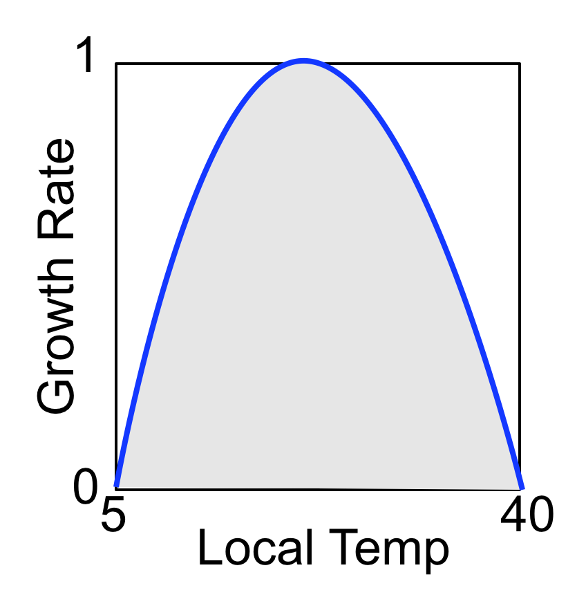
At the beginning of time, the planet is vacant -- no daisies. But the daisies will try to colonize the uncovered land as time goes on and as conditions become favorable for their growth. Each of the daisies has a preferred temperature range; they grow best at an optimum temperature and there are upper and lower temperature limits to the their growth. The model incorporates a growth factor that varies from 1 to 0, defined according the the following equation:
Growth Factorwhite = 1-0.003265(22.5-Twhite)2
The growth factor for the black daisies is calculated in a similar manner. This equation may look complex, but it is just a parabola, as shown in the figure below. This parabola has a peak value of 1 -- the maximum growth factor possible at an optimum temperature of 22.5°C -- and drops to zero at local temperatures of 5°C and 40°C. Thus, growth of the daisies can only occur within this temperature range, but remember that this is the local temperature.
Now we come to a key part of the model; the local temperature of the land around the two types of daisies will differ because of the fact that they absorb different amounts of solar energy. The black daisies absorb more energy and they radiate this energy, heating their surroundings. In contrast, the white daisies reflect more solar energy, which lessens the amount absorbed in that region, so that region ends up being cooler than if there were no white daisies. The local temperature is defined according to the following equation:
Twhite = FHA * (Aplanet-Awhite) + Tplanet
where A represents the albedo and FHA is the heat absorption factor, initially set at 20. This means that if the albedo of the planet is initially 0.5 and the albedo of the land with white daisies is 0.75, then the local temperature of the white land is 5°C cooler than the average planetary temperature. There is a similar equation for the local temperature of the black land, such that it is 5°C warmer than the planetary average.
Once the growth factors have been calculated, the model determines how much new area will be gained or lost by each daisy. The way this works is shown in the figure below, a simplified version of the more complex model we'll get to shortly.
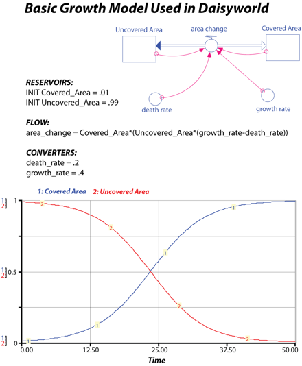
In the above figure, note that we use reservoirs to represent the areas. The flow connecting these area reservoirs is a biflow, meaning that area can be transferred in either direction -- the daisies may gain ground by taking it from the uncovered area reservoir, or they may lose ground, in which case area is added to the uncovered reservoir. The question of whether the daisies gain or lose land is a function of the growth factor, the death rate, and the area covered and also the area uncovered. In the form of an equation, we can represent this as follows:
area change = areadaisies*(areaun*growth factor - death rate)
This equation basically consists of two parts -- one that gives the area lost because of the natural death rate and one that gives the area gained due to growth of the daisies. The part that determines the area lost because of the natural death rate is pretty simple, but the other part is a bit more complex -- it will tend to be higher when the area covered is higher but also when the area uncovered is higher. The idea here is that with more land covered, there will be more daisies, producing more seeds that can spread out and successfully colonize the remaining land. But as the uncovered land declines, the success rate of seeds also declines because of overcrowding. The complexity here comes from the fact that area reservoirs are connected to each other and their sum at any point in time is equal to a constant value (1 in this case). As can be seen in the above figure, the result is that the rate of area change reaches a maximum when the there is an equal balance between land covered and land uncovered. This model represents a very simple ecosystem, but it is sufficient for the purposes of Daisyworld, which is, after all, a very simple model.
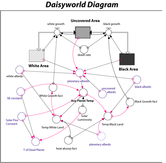
Now we are ready to dive into the real model. Use the model diagram and the equations below to construct a model of Daisyworld
Diagram of Daisyworld
As you create this model, be sure to make the two flows biflows, with the black arrows pointing to the Uncovered Area reservoir. To make a biflow, you first draw the flow, then double click the circle in the middle of the flow and click the biflow button in the upper left of the window. You can switch the black arrow back and forth from one reservoir to another by holding the control key down as you click on the black arrow. The black arrow signifies the direction of movement if the value is negative. Also note the ghosted planetary albedo converter in the lower right — define the one in the center of the diagram first and then transfer a ghost of it to the lower right; this is just to simply the diagram a bit and reduce the number of crossing connector arrows.
Equations for Daisyworld Model
Reservoirs: (make sure these are all non-negative by clicking the appropriate box)
INIT Uncovered_Area = 1.0 {portion of surface that daisies can occupy}
INIT Black_Area = 0
INIT White_Area = 0
Flows:
black_growth = Black_Area*(Uncovered_Area*Black_Growth_fact-death_rate)+.001 {the .001 is needed to give the system a bit of a nudge; without it the daisies never get going}
white_growth = White_Area*(Uncovered_Area*White_Growth_fact-death_rate)+.001 {the .001 is needed to give the system a bit of a nudge; without it the daisies never get going}
Converters:
Avg_Planet_Temp = ((Solar_Luminosity*Solar_Flux_Constant*(1-planetary_albedo)/SB_constant)^.25)-273 {energy balance to calculate temperature in °C}
black_albedo = .25
Black_Growth_fact = 1-.003265*((22.5-Temp_Black_Land)^2) {this is the equation for a parabola like that shown in Figure 8.03}
death_rate = 0.3
heat_absorp_fact = 20 {this controls how the local temperatures of the daisies differ from the average planetary temperature}
planetary_albedo = (Uncovered_Area*uncovered_albedo)+(Black_Area*black_albedo)+(White_Area*white_albedo)
SB_constant = 5.669E-8 {Stefan-Boltzmann constant W/°K^4}
Solar_Flux_Constant = 917 {W/m2 -- for reference, our Sun cranks out 1370 W/m2 }
Temp_Black_Land = heat_absorp_fact*(planetary_albedo-black_albedo)+Avg_Planet_Temp
Temp_White_Land = heat_absorp_fact*(planetary_albedo-white_albedo)+Avg_Planet_Temp
T_Dead_Planet = ((Solar_Luminosity*Solar_Flux_Constant*(1-.5)/SB_constant)^.25)-273 {energy balance to calculate temperature in °C of a planet with no dasisies}
uncovered_albedo = .5
white_albedo = .75
White_Growth_fact = 1-.003265*((22.5-Temp_White_Land)^2)
Solar_Luminosity = 0.6+(time*(1.2/200))
Be careful in assembling this model -- there is no steady state that we can use as a test of whether or not the model is properly constructed.
Experiments
1. The Standard Case
We'll begin our exploration of Daisyworld by looking at the standard case, with the model set up as originally described. This model is rather difficult to predict, so you should carefully study the model before forming a prediction of what will happen when you run it.
Remember that initially, there are no daisies on the planet (just a few seeds) and the sun's luminosity is very low. What will happen at first? Will the both types of daisies start to grow right away? Or just one type? What do we need to know in order to figure out whether or not the daisies will grow? We need to know the local temperature for each daisy. But to get the local temperature, we first need to know the average planetary temperature. We can in fact figure out the starting temperature for Daisyworld using the following equation:
Tplanet = (Solar Energy * (1-Aplanet)/s)0.25 - 273
At the start of the experiment, the solar energy is found by multiplying the luminoisty (0.6) times the solar flux constant (917 W/m2); the planetary albedo is 0.5 (no daisies); and s is 5.669E-8 W/°K4, so the planetary temperature is about -9°C in the beginning. This means that the local temperature for the black daisies (if there were any) would be -4°C and for the white daisies, it would be -14°C -- both of these temperatures are too cold for the daisies to grow, so initially, the daisies will be incapable of altering the albedo and thus the planetary temperature. This gives us a starting point for developing a prediction about what will happen, but there are many more questions to think about before running this model.
But what will happen as the planet begins to warm, driven by the increasing energy output of the sun? Which type of daisy will begin to grow first? What will happen to the planetary temperature when the first daisies begin to grow? How will that change in the planetary temperature change the growth of the daisies. Will both types of daisies grow during the same time period? If so, what will be their combined effect on the planetary temperature?
Run the model for 200 time units, with a DT of 0.25. It will be instructive to plot the three area reservoirs on one graph, and the average planetary temperature and the temperature of the "dead" planet on another graph. Various other graphs will be necessary to fully understand what is going on to drive the observed behavior.
2. Changing Albedos
Initially, the black albedo is set at 0.25, while the white albedo is 0.75. In this experiment, modify these albedos, first to more extreme values (.05 and .95) and then to more moderate values (.4 and .6). Be sure to make some careful predictions before running these models.
3. Changing Growth Factor Curve
One of the critical parts of this model is the growth factor for daisy growth. In this experiment, we will alter the growth factor and see how the model responds.
a) First, alter the optimum temperature for the daisies' growth, which is initially set at 22.5°, to 15°. To do this, alter the equations for the growth factors, replacing 22.5 with 15. As always, make predictions before running the model.
b) Next, restore the optimum temperature to 22.5 and then reduce the range of temperatures that the daisies can tolerate. Initially, the daisies can grow in temperatures ranging from 5 to 40. Now restrict the range so that the daisies grow only between 18 and 27; this can be done by replacing the 0.003265 with 0.05 in the equations for the growth factors. As always, make predictions before running the model.
4. Plagues
This experiment explores the resilience of Daisyworld by programming a set of plagues into the model. These plagues decimate the populations periodically for brief periods. An interesting question here is whether or not the daisies will be able to recover fast enough to return the planetary temperature to the "comfort zone". To implement this change, double-click on the death rate converter and replace 0.3 with "time" (without the quotation marks), then click on the Become Graph button in the lower left of the window. Next set the number of data points to 101; this should give you one input value every 2 time units, thus allowing us to make fairly brief plagues (still, these are 20 Myr long!). Then, select the entire output column by clicking directly on the word "Output" at the top of the column and enter 0.3, then click on one of the other boxes in the graph window to register this change -- this should set the background death rate to 0.3. Next, scroll along the horizontal axis and make a spike with a value of 1.0 at time units 50, 100, and 150; click on the OK button and the plagues should be inserted into the model. Run the model as before, after making a prediction about what will happen. Are all of the plagues equal in magnitude (in terms of area lost as a result of the deaths)? Does each plague result in the same kind and magnitude of temperature change? Does the system recover from each plague? What determines whether or not the planet recovers from a plague?